Sign In
September 23, 2024
Tables in Python made easy for engineers with Pandas

by Thomas Nagels

Build successful applications
Learn how you (developer, engineer, end-user, domain expert, project manager, etc.) can contribute to the creation of apps that provide real value to your work.
What are tables in Python?
In Python, you can store your data in multiple ways. Although there aren’t any ‘tables’ as you would have in a database, you can leverage the structures that resemble tables or manage tabular data. In Python, most programmers will be familiar with (nested) lists simulating columns and rows, dictionaries that represent rows of data with named columns (also known as the key), and the Pandas DataFrame.
For the examples in this blog, we will use Pandas. There are many more ways you can order your data in tabular formats, so make sure you use the structure that is best for your data manipulation and storage methods.
Advantages of dedicated tables in Python over lists
Although the built-in data types in Python are great, Pandas is still preferred because of three main reasons:
-
Easy data manipulation: Pandas has functions for filtering, grouping, merging and so much more that make it much easier compared to handling these operations with lists or dictionaries in Python.
-
Better performance: A Pandas DataFrame is optimized for performance, and this becomes apparent when dealing with large amounts of data. It uses efficient data structures under the hood that will outperform pure Python lists and dictionaries.
-
Rich analytical tools: Pandas easily integrates with other libraries and has become a hit with other software too. When it comes to analyzing, visualizing, and exporting data, Pandas is king.
Examples in AEC where you could use a table
For most engineers, tables are everywhere. Suffice it to say, the same goes for a geotechnical engineer. A simple example is for presenting soil test results. In this scenario, we have soil test results from multiple boreholes (depth, moisture, content, shear strength, etc) in a tabular format. Coupled with a DataFrame, you can quickly filter properties, enabling an efficient comparison and analysis.
Creating and manipulating tables
Next, you will learn how to quickly make yourself a table and go over some of the most important methods for an Engineer. If you are familiar with Pandas you can skip this section. 😉
Making a table with Python from scratch
Let's use the first example from the previous section to become familiar with the basic methods of Pandas. Before you can start coding with Pandas you must not forget to ‘pip install pandas’ in your Windows PowerShell or terminal.
Now, you can open a .py file and start coding! As always, you start by importing pandas.
1import pandas as pd
The next step is to use the pd.DataFrame() and create your first table:
1Data  = pd.DataFrame({
2
3    'Borehole': ['BH1', 'BH2', 'BH1', 'BH2'],
4
5    'Depth': [5, 12, 15, 20],
6
7    'Moisture_Content': [15, 12, 18, 14],
8
9    'Shear_Strength': [100, 120, 110, 130]
10
11})
Let's say you want to extend the measurements DataFrame to contain the measurements of borehole s3. In this case, you can simply use the following code to extend the DataFrame.
1data.loc[len(data)] = [‘BH3’, 8, 20, 115] 3 First row for BH3
2
3data.loc[len(data)] = [‘BH3’, 16, 22, 125] # Second row for BH3
If you discover the data for your borehole measurement to be incorrect, you can easily replace it by using the following line of code.
1df.loc[(df[‘Borehole’] == ‘ BH2’) & (df[‘Depth’] == 10), ‘Depth’ ] = 12
In short, this line of code first selects all the rows where the borehole is BH2 and then targets the specific row where the depth is 10 meters, finally replacing the value.
So what if you print this DataFrame, what will it look like? Well, like a table!
| Borehole | Depth | Moisture Content | Sheer strength |
|---|---|---|---|
| BH1 | 5 | 15 | 100 |
| BH2 | 10 | 12 | 120 |
| BH1 | 15 | 18 | 110 |
| BH2 | 20 | 14 | 130 |
| BH3 | 8 | 20 | 115 |
| BH3 | 16 | 22 | 125 |
Just like a table in Excel your table has rows and columns, and you can use the titles and indexes to find values.
Now that you know how to make a table and modify it, let's look at some of the methods that could be interesting for an engineer to extract data from a file.
How to extract data from a file
In all fields of engineering, data often comes in various file formats. Being able to convert file types without the loss of data is key. In this section, we will quickly go over some common file formats and convert them into a pandas DataFrame in just two lines or less!
- .csv and .txt files: widely used for tabular data such as material properties, load cases, or test results. Add the correct delimiter to the arguments for text files and you can use the same method!
1df = pd.read_csv(‘data.csv’)
2
3df = pd.read_csv(‘data.csv’, delimiter=‘\t’) # For tab-seperated text
- Excel files: Often used for larger data sets such as soil test results, structural analysis outputs, or project cost sheets, the caveat here being that there are multiple sheets.
1df = pd.read_excel(‘data.xlsx’, sheet_name=’Sheet1’)
- JSON files: May be used for data interchange or storing complex data such as 3D model parameters or test results.
1df = pd.read_json(‘data.json’)
- SQL Database(.db & .sqlite): For managing large-scale project data or geotechnical borehole databases. The small caveat being that you need to connect to the database.
1conn = sqlite3.connect(‘database.db’)
2
3df = pd.read_sql_query(“SELECT * FROM table_name”, conn)
As you may have noticed, most of these methods are built into Pandas. The same methods exist for XML, HDF5 and many more file formats, proving that Pandas is a great package for engineers to use for their workflows!
Analyzing data with tables
When you look up Pandas you will find that it is a popular open-source data analysis and manipulation library for Python. Through Pandas, you can leverage methods that may not be aimed at engineering to our advantage.
Data exploration
Filtering and analysis are great ways to become familiar with and understand your data. Did you just receive a data set from a colleague, and would you like to take a look at what they measured? Then you can use the .head() to see the first 5 rows of a DataFrame and .info() will provide the information on the data types, column names, and missing values which is critical for understanding the quality of the data.
Once you understand the data, you may want to inspect some values before performing calculations. You can use filtering to access certain sections of your dataset.
Let's use the borehole example: an engineer may want to focus on data from specific boreholes or depths. Possibly a shallow layer to inspect the soil properties or use them in an analysis later. Here are two quick examples to filter:
1#By borehole
2
3borehole_data = df[df[‘Borehole’] == ‘BH1’]
4
5#By depth Range
6
7shallow_data = df[df[‘Depth’] <= 10]
Would you like to sort the data that you just filtered on? You can easily sort your new DataFrame by depth using the .sort_values method:
1sorted_shallow_data = shallow_data.sort_values(by=‘Depth’)
The Geotechnical Engineer now has their data in a logical order, helping to visualize the sequence of measurements at different soil layers.
Simple data analysis
Some simple data analysis can give an engineer some key insights. For the previous example, you can calculate some subsurface conditions, helping to inform design decisions, safety assessments, and project planning. Here are two examples that may be useful relating back to the borehole example:
- Identifying soil strength variation with depth: by analyzing the shear strength values at different depths, you can identify changes in the soil stability. This will help the geotechnical engineer locate weak soil layers and where reinforcement or further investigation may be needed before construction can proceed.
1#Group by depth and calculate the average shear strength at each depth
2
3avg_shear_by_depth = df.groupby(‘Depth’)[Shear_Strength’).mean()
- Detecting anomalies in borehole data: identifying outliers or anomalies is key to finding unusual subsurface conditions or data entry errors which may affect the process of construction drastically. Unusually high shear strength at a certain depth may indicate the presence of a dense rock layer.
1# Detect outliers in shear strength using a threshold
2
3Outliers = df[df[‘Shear_Strength’] > df[‘Shear_Strength’].mean() + 2 * df[‘Shear_Strength’].std()]
These simple analyses enhance a geotechnical engineer's understanding of the environment, allowing for more informed decision-making on soil behaviour, stability, and potential construction challenges.
Visualizing Pandas table data
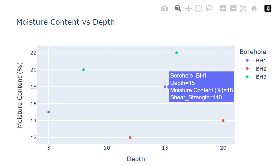
Once you have our key insights, you can support them with an interactive visual. For this, you can leverage the power of Plotly. It is one of the many packages that work effortlessly with Pandas. The following code snippet will use the original borehole data and create an interactive plot.
1fig1 = px.scatter(table, x='Depth', y='Moisture_Content', color='Borehole',
2
3                 labels={'Moisture_Content': 'Moisture Content (%)'},
4
5                 title='Moisture Content vs Depth',
6
7                 hover_data=['Shear_Strength'])
8
9fig.show()
Some of the benefits of Plotly for Pandas is the out-of-the-box interactiveness that Plotly offers for Pandas DataFrames. You can – as displayed in the graph – hover over data to see additional information. You can zoom and pan in on data and have the boreholes color-coded, meaning if you have many measurements, you can even ‘turn off’ other data and see trends in the moisture across the depth of the borehole! You may find that Excel can do this too, but can it do all this in such a small amount of time/operations?
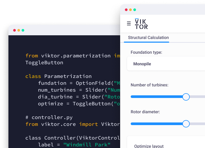
Building an engineering application with VIKTOR’s TableView
Building applications is a great way to make your code available to many users at the same time. You can easily make a simple application from the borehole example using VIKTOR’s TableView and PlotlyAndDataView in a mere 65 lines of code.
The application will let the user upload their data, extend the data if they have additional data, and see a simple analysis on the data in a plot and data overview.
Want to see the result? You can test it using this link.
You begin by using the following command in your terminal to create an app template:
1>viktor-cli create-app –app-type editor .
You will then add Plotly and Pandas to your requirements.txt file so that it looks like this:
1viktor==14.15.2
2pandas
3plotly
The next step is to install and start your app using the following command in your terminal:
1>viktor-cli clean-start
This may take a few minutes so feel free to grab a cup of coffee in the meantime!
Once you see that the app is ready, you can begin making your app. Open app.py and you will see one import and two classes are already present in the file.
You will add two imports yourself, Pandas and Plotly:
1import viktor as vkt
2
3import pandas as pd
4
5import plotly.express as px
You can then move your focus to your Parameterization in which you define all your inputs. You want the user to be able to upload their data so you will create an input called a FileField in which the user can upload their .csv file.
1class Parametrization(vkt.Parametrization):
2
3    input_file = vkt.FileField('Upload a .CSV file', file_types=['.csv'], max_size=500_000)
As you can see, you have constrained the allowed file types to .csv and a maximum size of 500MB.
Next, you also want to let a user add data to extend the set of measurements. For this, you will use a DynamicArray with some NumberFields for the values. To prevent a user from entering infeasible values you will constrain the allowable range of numbers using minimum and maximum values.
1class Parametrization(vkt.Parametrization):
2
3    input_file = vkt.FileField('Upload a .CSV file', file_types=['.csv'], max_size=500_000)
4
5    extend_data = vkt.DynamicArray('Add measurement')
6
7    extend_data.borehole = vkt.NumberField('Borehole: ', default=1, min=1, step=1)
8
9    extend_data.depth = vkt.NumberField('Depth (m): ', default=1, min=1)
10
11    extend_data.moisture_content = vkt.NumberField('Moisture Content (%): ', default=15, min=1, max=100)
12
13    extend_data.shear_strength = vkt.NumberField('Shear Strength (N/m^2)', default=100, min=1)
Those are all your input parameters done! Let's start making some functions for the views.
You will start by writing a function to display and extend the data. For this, you will begin by writing a function to convert the uploaded .csv file into a pandas DataFrame. Should a user not have an input file, you will also add the DataFrame you made earlier as a default value.
Your function to initialize the data will look like this:
1class Controller(vkt.Controller):
2
3    parametrization = Parametrization
4
5
6
7    def initialise_data(self, params):
8
9        input_file = params.input_file
10
11        if input_file:
12
13            csv_file = input_file.file
14
15            with csv_file.open() as r:
16
17                measurements = pd.read_csv(r)
18
19        else:
20
21            measurements = pd.DataFrame({
22
23            'Borehole': ['BH1', 'BH2', 'BH1', 'BH2', 'BH3', 'BH3'],
24
25            'Depth': [5, 12, 15, 20, 8, 16],
26
27            'Moisture_Content': [15, 12, 18, 14, 20, 22],
28
29            'Shear_Strength': [100, 120, 110, 130, 115, 125]
30
31            })
32
33        return measurements
In this function, you use the parameters from the parametrization to access the input file. You then check for a file and if there is one, you extract the data from it using the pd.read_csv() from earlier!
If not, you use the measurement data from before. It is good practice to always have a default for your apps such that when a user opens your app, they are never confronted with nasty errors.
Next, you can write a function to extend your pandas DataFrame like you did earlier:
1def extend_measurements(self, params):
2
3        new_data = params.extend_data
4
5        measurements = self.initialise_data(params)
6
7        if new_data:
8
9            for entry in new_data:
10
11                measurements.loc[len(measurements)] = [f'BH{entry['borehole']}',
12
13                                                       entry['depth'],
14
15                                                       entry['moisture_content'],
16
17                                                       entry['shear_strength']]
18
19        return measurements
Here, you use the function you just made to initialize your data. Should there be an entry for new data in your parameters (params), you extend your measurements accordingly, just like you did earlier.
Now let's display this data in a Table! You can create a third function for your table in Python. This will be a very simple one because everything is set up in your pandas DataFrame so you do not need to worry about anything anymore and let VIKTOR display your beautiful table like this:
1class Controller(vkt.Controller):
2
3    parametrization = Parametrization
4
5...
6
7    @vkt.TableView('Table of Measurements')
8
9    def table_of_measurements(self, params, **kwargs):
10
11        table = self.extend_measurements(params)
12
13        return vkt.TableResult(table)
Now is also a great time to open your app in the environment and take a look at the result. If all went well, you should have something like this:
If you add a new row for borehole 4, you see it appears in the table instantly. The TableView also lets you download the result so any changes you make can immediately be downloaded.
Now let's also add an interactive plot and one of the insights to your application.
To calculate the insights into the average shear strength per depth, you can simply write another function:
1class Controller(vkt.Controller):
2
3    parametrization = Parametrization
4
5...
6
7    def calculate_avg_shear_by_depth(self, params):
8
9        measurements = self.extend_measurements(params)
10
11        avg_shear_by_depth = measurements.groupby('Depth')['Shear_Strength'].mean()
12
13        return avg_shear_by_depth
Once again, you initialize your data and use the power of Pandas to calculate the average shear strength by depth.
Now you can create the plot and data overview in your application. There are two parts to this view, the plot and the data:
1 @vkt.PlotlyAndDataView('Plot and Analysis')
2
3    def plot_analysis(self, params, **kwargs):
4
5        table = self.extend_measurements(params)
6
7        #make plot:
8
9        fig1 = px.scatter(table, x='Depth', y='Moisture_Content', color='Borehole',
10
11                 labels={'Moisture_Content': 'Moisture Content (%)'},
12
13                 title='Moisture Content vs Depth',
14
15                 hover_data=['Shear_Strength'])
16
17        fig1.update_traces(marker=dict(size=12))
18
19        #Data insight:
20
21        avg_shear_by_depth = self.calculate_avg_Shear_by_depth(params)
22
23        viktor_data = []
24
25        for index in avg_shear_by_depth.index:
26
27            item = avg_shear_by_depth.loc[index]
28
29            viktor_data.append(vkt.DataItem(f'Average shear strength at {index} meter:', item, suffix='N/m^2'))
30
31        data = vkt.DataGroup(*viktor_data)
32
33        return vkt.PlotlyAndDataResult(fig1.to_json(), data)
For this function, you can see that the plot made earlier is used again and for better visibility you increased the size of the markers.
You then use the function you just wrote to calculate the average shear strength by depth and display each depth and its corresponding shear strength in a VIKTOR DataItem. The result looks like this:
And that is it! You now have a working app that you can use to upload, inspect, extend and analyze the borehole data using the power of Pandas and VIKTOR! If you enjoyed this blog and would like to learn more about VIKTOR apps you can visit the Apps Gallery, get the free version or book a demo with one of our experts!
If you would like the full code for this app, you can find it below:
1import viktor as vkt
2import pandas as pd
3import plotly.express as px
4
5class Parametrization(vkt.Parametrization):
6    input_file = vkt.FileField('Upload a .CSV file', file_types=['.csv'], max_size=500_000)
7    extend_data = vkt.DynamicArray('Add measurement')
8    extend_data.borehole = vkt.NumberField('Borehole: ', default=1, min=1, step=1)
9    extend_data.depth = vkt.NumberField('Depth (m): ', default=1, min=1)
10    extend_data.moisture_content = vkt.NumberField('Moisture Content (%): ', default=15, min=1, max=100)
11    extend_data.shear_strength = vkt.NumberField('Shear Strength (N/m^2)', default=100, min=1)
12
13class Controller(vkt.Controller):
14    parametrization = Parametrization
15
16    def initialise_data(self, params):
17        input_file = params.input_file
18        if input_file:
19            csv_file = input_file.file
20            with csv_file.open() as r:
21                measurements = pd.read_csv(r)
22        else:
23            measurements = pd.DataFrame({
24            'Borehole': ['BH1', 'BH2', 'BH1', 'BH2', 'BH3', 'BH3'],
25            'Depth': [5, 12, 15, 20, 8, 16],
26            'Moisture_Content': [15, 12, 18, 14, 20, 22],
27            'Shear_Strength': [100, 120, 110, 130, 115, 125]
28            })
29        return measurements
30
31    def extend_measurements(self, params):
32        new_data = params.extend_data
33        measurements = self.initialise_data(params)
34        if new_data:
35            for entry in new_data:
36                measurements.loc[len(measurements)] = [f'BH{entry['borehole']}',
37                                                       entry['depth'],
38                                                       entry['moisture_content'],
39                                                       entry['shear_strength']]
40        return measurements
41
42    def calculate_avg_shear_by_depth(self, params):
43        measurements = self.extend_measurements(params)
44        avg_shear_by_depth = measurements.groupby('Depth')['Shear_Strength'].mean()
45        return avg_shear_by_depth
46
47    @vkt.TableView('Table of Measurements')
48    def table_of_measurements(self, params, **kwargs):
49        table = self.extend_measurements(params)
50        return vkt.TableResult(table)
51
52    @vkt.PlotlyAndDataView('Plot and Analysis')
53    def plot_analysis(self, params, **kwargs):
54        table = self.extend_measurements(params)
55        #make plot:
56        fig1 = px.scatter(table, x='Depth', y='Moisture_Content', color='Borehole',
57                 labels={'Moisture_Content': 'Moisture Content (%)'},
58                 title='Moisture Content vs Depth',
59                 hover_data=['Shear_Strength'])
60        fig1.update_traces(marker=dict(size=12))
61        #Data insight:
62        avg_shear_by_depth = self.calculate_avg_Shear_by_depth(params)
63        viktor_data = []
64        for index in avg_shear_by_depth.index:
65            item = avg_shear_by_depth.loc[index]
66            viktor_data.append(vkt.DataItem(f'Average shear strength at {index} meter:', item, suffix='N/m^2'))
67        data = vkt.DataGroup(*viktor_data)
68        return vkt.PlotlyAndDataResult(fig1.to_json(), data)
Conclusion - Tables with Python
Being able to create, modify and analyze tables with Python is a game changer for engineers. Although Pandas is designed for the data science community, it opens many doors for engineers too. Thanks to its simplicity and well-designed package, an engineer does not need extensive Python knowledge to get started. As you've learned, building VIKTOR apps is easy and you can leverage the TableView to display your tables and calculations in an interactive way.
Start building apps for free
Related Blog Posts

Get our best content in your inbox
Subscribe to our newsletter and get the latest industry insights