How to calculate cross-section properties using Python

Analyzing cross-sections can be one of the more challenging aspects of a structural engineer's work. Detailed calculations of area, moments of inertia, centroids, radii of gyration, and section modulus require time and effort, and traditional tools are often not easy to use or accessible. These properties are crucial in:

• Structural Design: Properties like area and moments of inertia help determine the section's ability to resist bending and compression.

• Stability Analysis: Radii of gyration and centroids help assess column stability and stress distribution.

• Finite Element Analysis (FEA): Moments of inertia and centroids are needed to create accurate models for analysis.

Structural analysis with SectionProperties

Fortunately, SectionProperties, an open-source Python package developed to help engineers perform these calcluations quickly, is here to change that.

In this blog, you will learn how to get started with this tool and how it could transform your workflow.

Installing SectionProperties

Installing SectionProperties is as simple as running the following command in your terminal:

pip install sectionproperties 

Calculating properties and analyzing cross-sections

Below, we will outline the basic workflow for using SectionProperties to calculate properties and analyze a cross-section.

First, we import the specific modules we will need.

Material allows us to define mechanical properties of materials, Geometry lets us import or define the geometry of a section, and Section is responsible for analyzing the section, such as calculating its geometric properties and generating stresses.

1from sectionproperties.pre import Material 
2from sectionproperties.pre.geometry import Geometry 
3from sectionproperties.analysis.section import Section 
4import matplotlib.pyplot as plt 

Next, we define a material for our section. In this case, we will use concrete:

1concrete = Material( 
2    name="Concrete", 
3    elastic_modulus=30.1e3,  # MPa 
4    poissons_ratio=0.2, 
5    density=2.4e-6,          # kg/mm³ 
6    yield_strength=32,       # MPa 
7    color="lightgrey") 

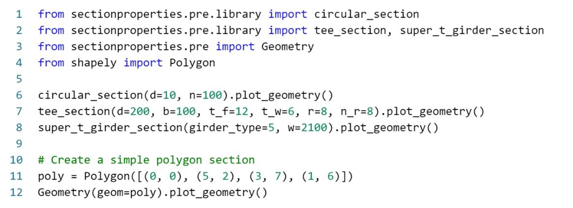
The SectionProperties library provides built-in functions to create typical cross-sections such as:

• Steel Sections: channel section, circular hollow section, angle_section, etc.

• Concrete Sections: concrete tee section, concrete circular section, etc.

• Bridge Sections

These functions are very useful for quickly defining typical structural cross-sections.

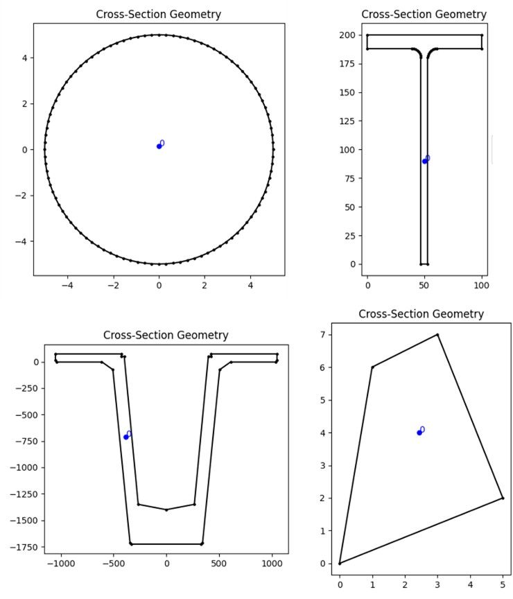
However, for more complex sections, it can be challenging to define them directly through code.

It is often easier to draw the section in AutoCAD or similar software and export it as a .dxf file, which can then be imported for analysis.

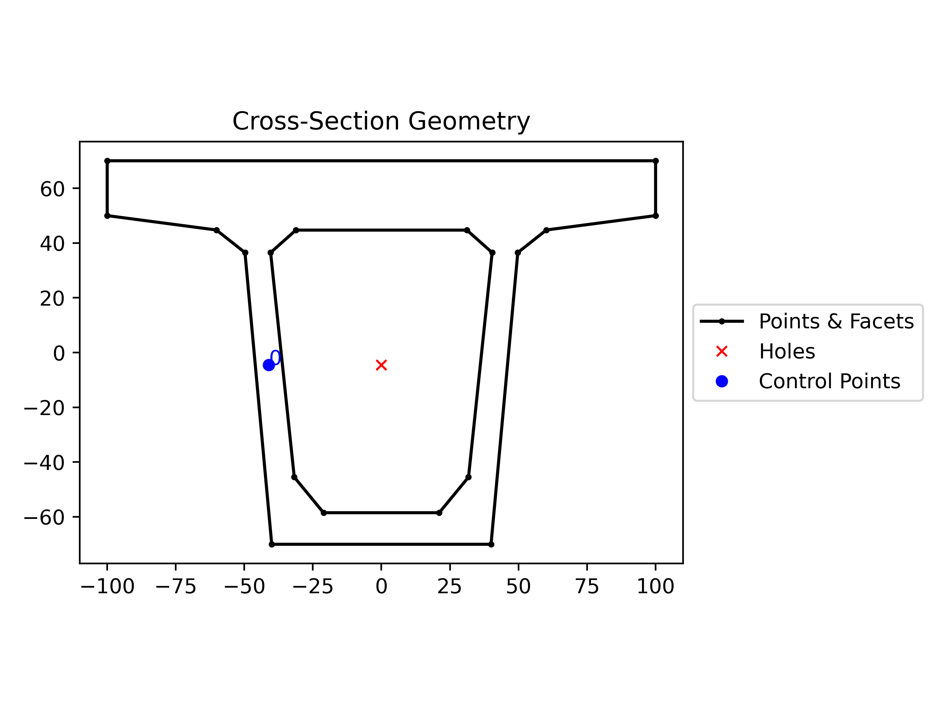
We import the geometry of our section, which represents a box girder bridge, from a .dxf file and associate it with the defined material:

1geom = Geometry.from_dxf(dxf_filepath="seccion1.dxf") 
2geom.material = concrete 
3geom.plot_geometry() 

Meshing is a crucial step in finite element analysis. It directly impacts the accuracy and reliability of the results.

Balancing mesh density is key: a fine mesh can improve accuracy, especially in critical areas, but also increases computational effort. We create the mesh for the section with the following code:

1geom.create_mesh(mesh_sizes=30) 
2sec = Section(geom) 
3# sec.display_mesh_info() 
4sec.plot_mesh() 
5plt.show() 

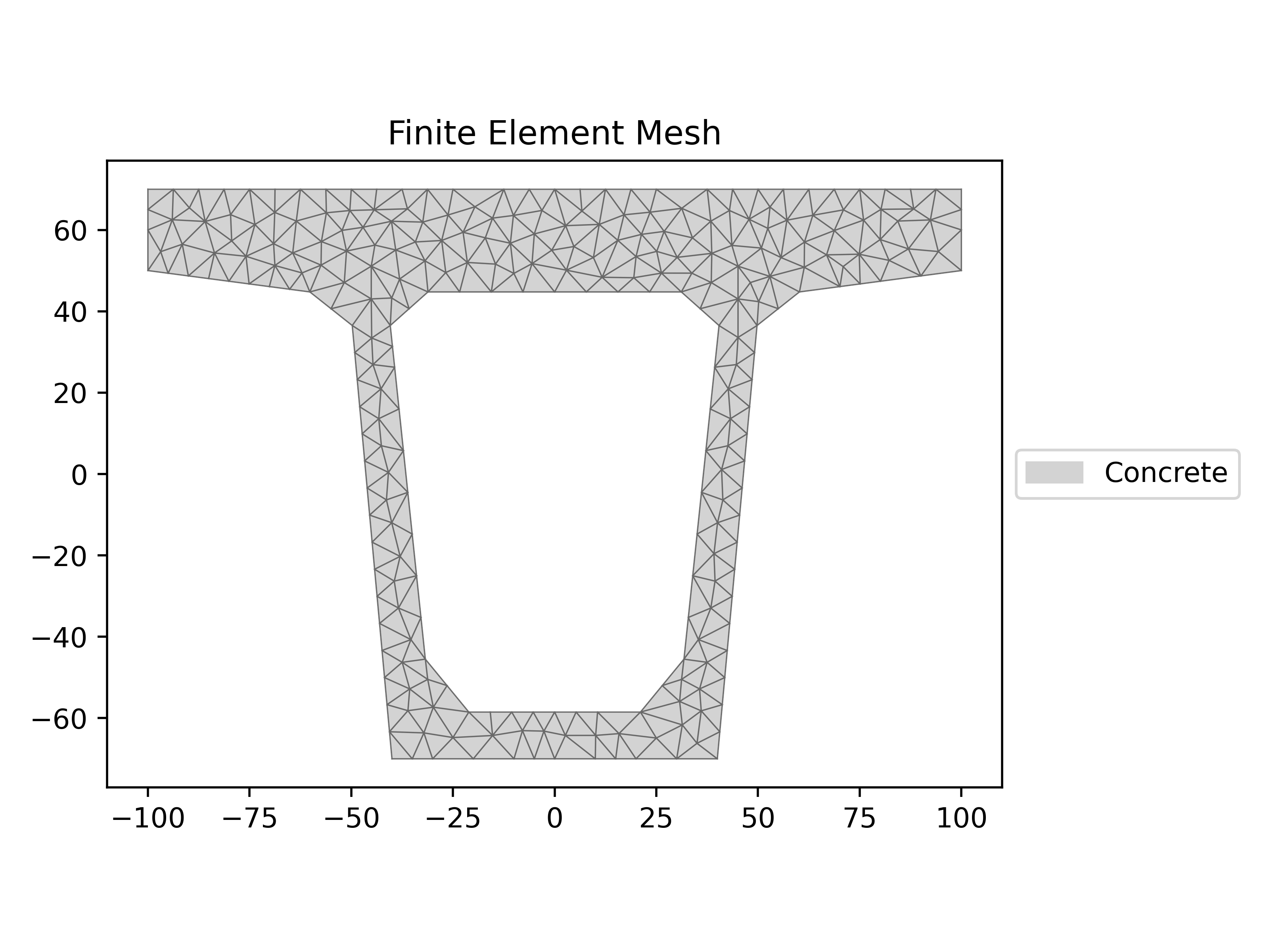
It is possible to control the mesh size using the mesh_sizes parameter, allowing us to achieve better accuracy, control computational cost, and analyze complex sections.

Visualizing the mesh allows us to verify that the discretization is adequate before proceeding with the calculations.

Calculating geometric- and warping properties

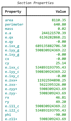
Once we have generated the mesh, we can calculate the geometric- and warping properties of the section:

1sec.calculate_geometric_properties() 
2sec.calculate_warping_properties() 
3sec.calculate_plastic_properties() 
4sec.display_results(fmt=".2f") 

These calculations allow us to obtain important information, such as area, moments of inertia, and centroid coordinates. Below are some of the results obtained:

Stiffness calculations

To calculate the axial, flexural, and torsional stiffness of the section and understand how it will respond to different types of loads, we use the following code:

1ea = sec.get_ea() 
2eixx, _, _ = sec.get_eic() 
3ej = sec.get_ej() 
4gj = sec.get_g_eff() / sec.get_e_eff() * ej 
5
6print(f"Axial rigidity (E.A): {ea:.3e} N") 
7print(f"Flexural rigidity (E.I): {eixx:.3e} N.mm2") 
8print(f"Torsional rigidity (G.J): {gj:.3e} N.mm2") 

Plotting centroids

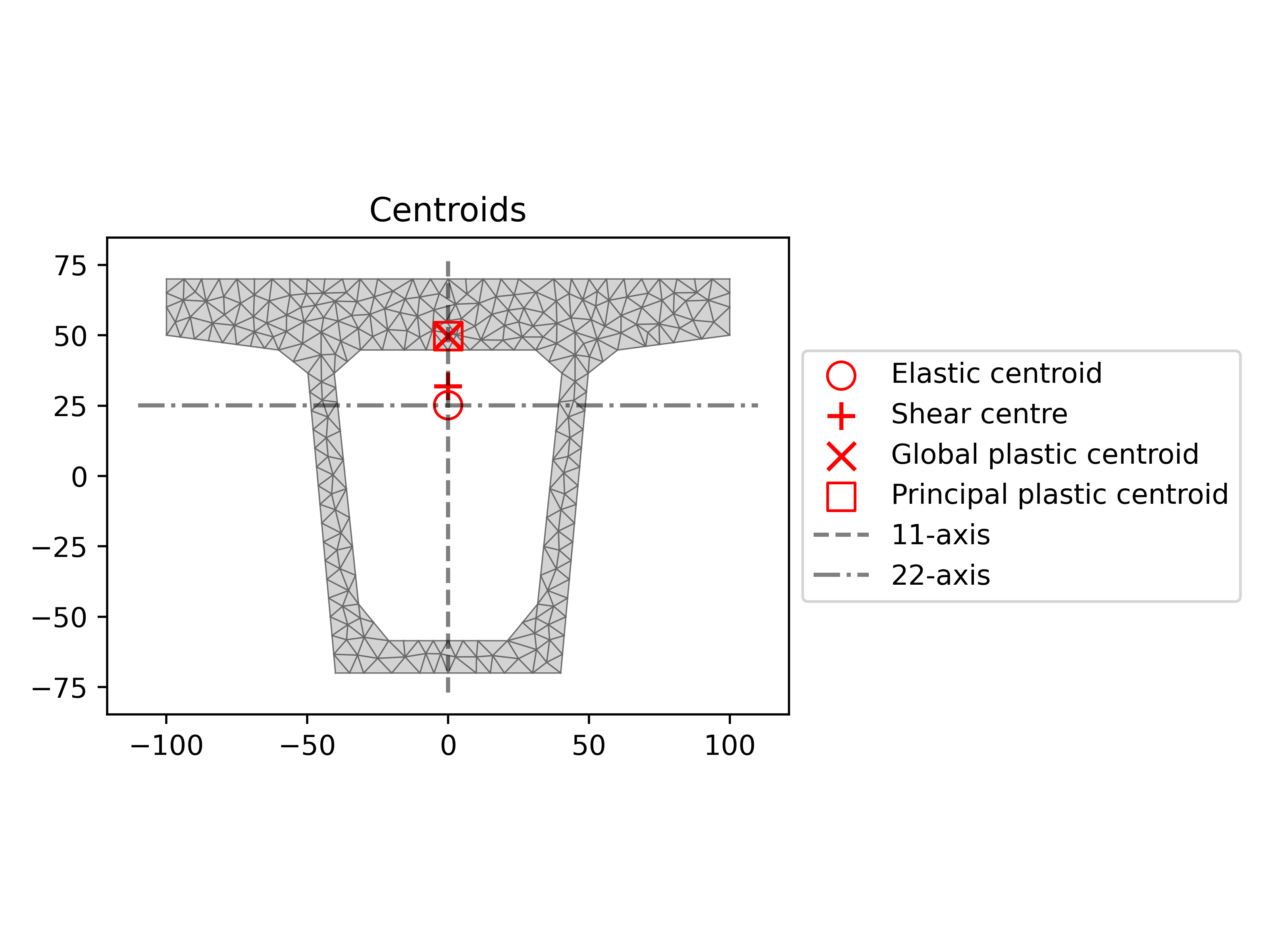
Additionally, we can visualize the elastic centroid, shear center, global plastic centroid, and principal axes to better understand the geometric distribution and structural behavior:

1sec.plot_centroids() 

Stress visualization

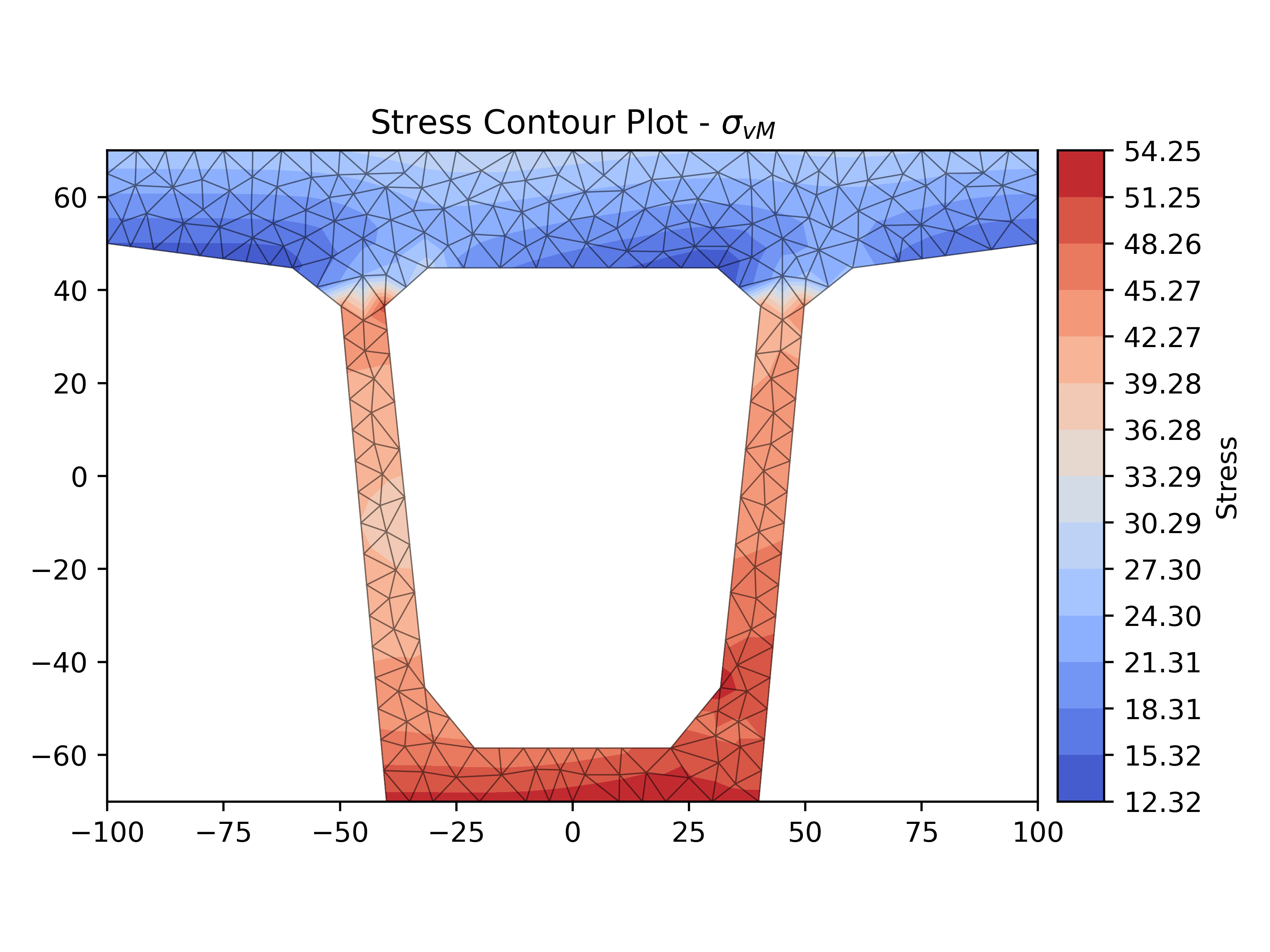
Finally, we can calculate and visualize the stresses. The cross-section being analyzed belongs to the central span of a simply supported beam. This beam is subjected to a combination of external loads, resulting in various types of stresses in the section:

n = 10e3 N, Axial load

mxx = 10e6 N-mm, Bending moment about the x-axis

vx = 25e3 N, Shear force in the x direction

vy = 50e3 N, Shear force in the y direction

We use this code to plot the Von Mises stresses in the section:

1stress = sec.calculate_stress(n=10e3, mxx=10e6, vx=25e3, vy=50e3) 
2stress.plot_stress(stress="vm", normalize=False, fmt="{x:.2f}") 

We can also use the following code to plot the shear stress vectors in the y direction:

1stress.plot_stress_vector(stress="vy_zxy", fmt="{x:.2f}") 

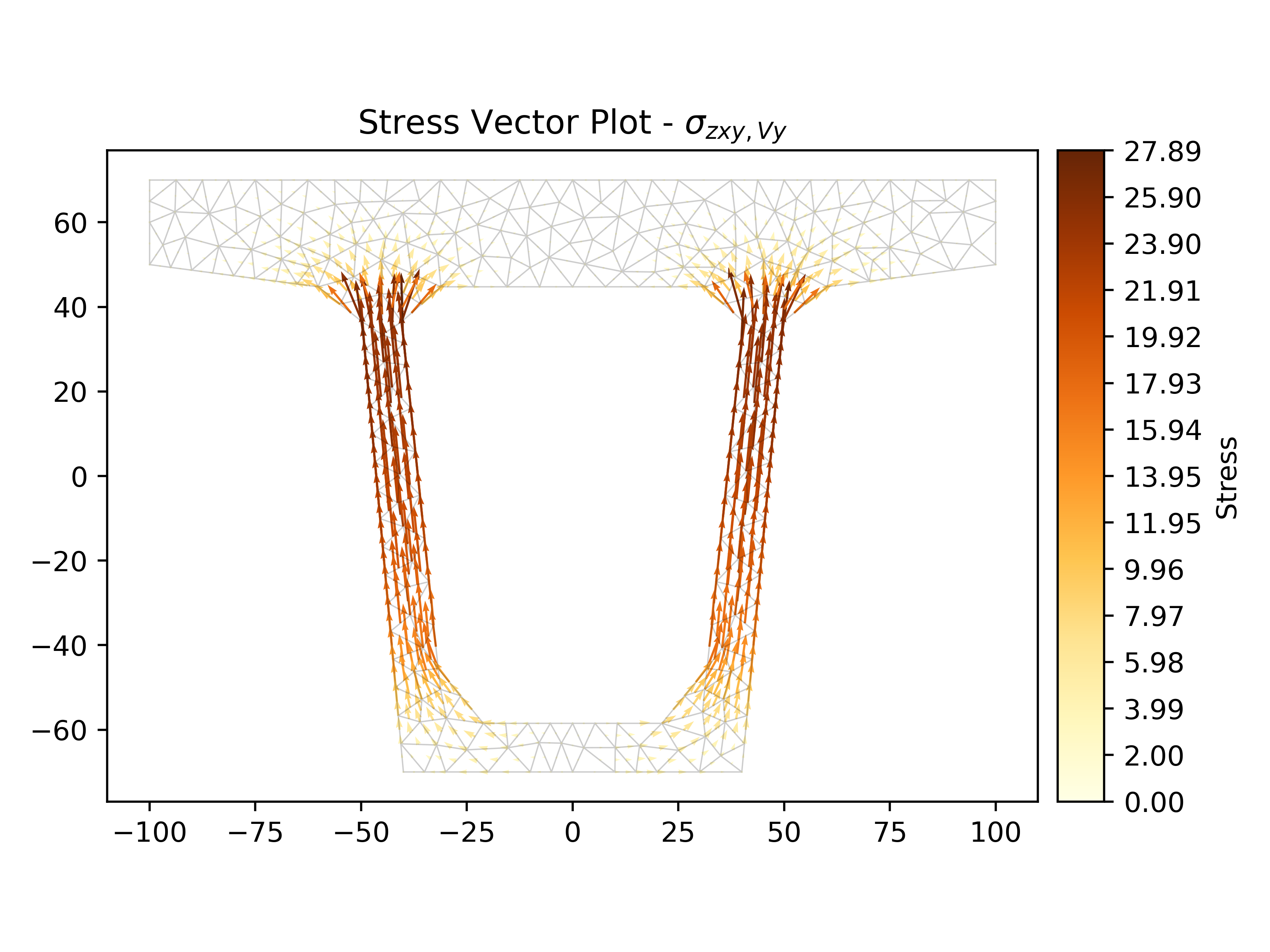
This way, we can visualize how shear stresses are distributed, where they act, and their values, allowing us to identify critical points and potential failure areas due to shear.

Lastly, we can plot Mohr's Circle to visualize the stress state at a specific point in the section located at coordinates x = 45, y = 40.

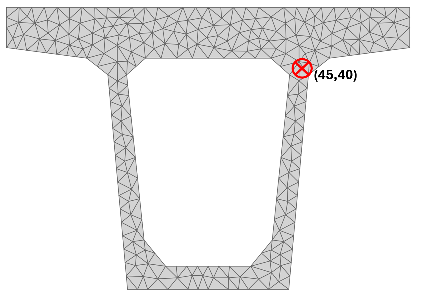
1stress.plot_mohrs_circles(x=45, y=40) 
2plt.show() 

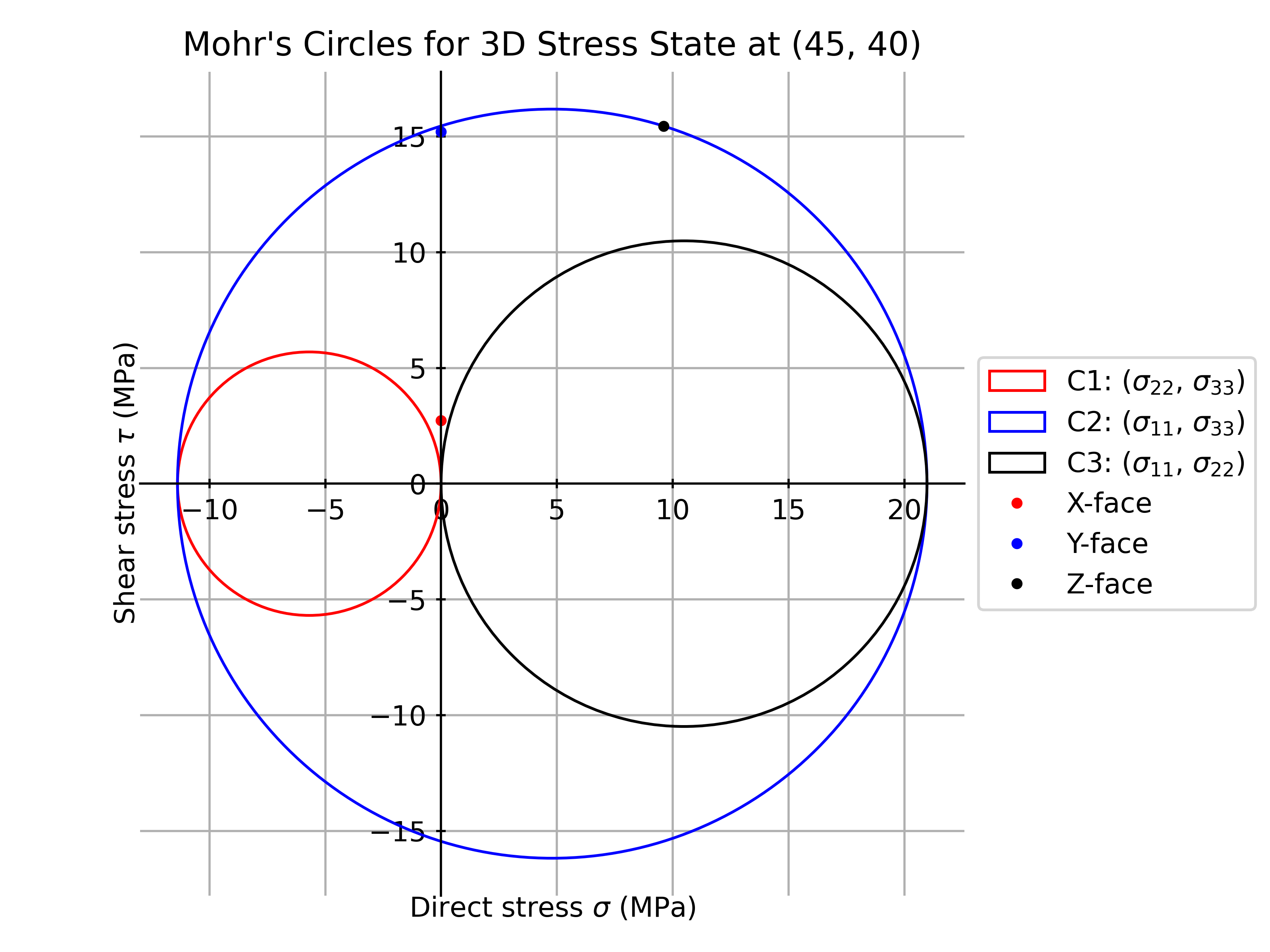
Mohr's Circle helps us visualize how principal and shear stresses relate to each other at a specific point in the section, also finding the maximum and minimum stress values and the orientations of the planes where they occur, helping to evaluate whether the section can withstand the applied loads without failing.

Turning SectionProperties into a tool

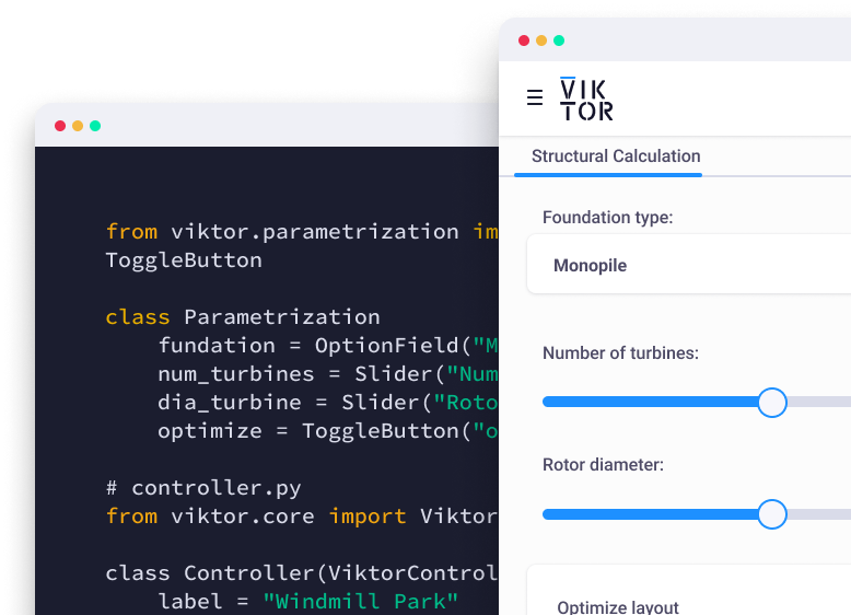
But what happens when you want to share your section analysis with other engineers if they don't know any Python? This is where you need a platform to turn your script into a user-friendly and accessible tool, like VIKTOR!

To show you how, we will now go through the process of turning a Python script that uses sectionproperties into an interactive web application that anyone can use.

Let's get started!

If you would like to give this application a go, feel free to try it here:

Step 1: Prepare the Parameters

It is important to define the parameters that the user can adjust. We will use NumberField, FileField, and OptionField, allowing users to input numerical values, upload .DXF files containing the section geometry, and select the type of analysis they wish to perform.

1class Parametrization(vkt.Parametrization): 
2    title1 = vkt.Text("## Material property") 
3    E = vkt.NumberField('Elastic modulus', default=30.1e3, flex=35, suffix="MPa") 
4    fc = vkt.NumberField('Yield strength', default=32, flex=35, suffix="MPa") 
5
6    title2 = vkt.Text("## Define Section") 
7    dxf = vkt.FileField('Upload DXF file', file_types=['.dxf'], flex=40) 
8    mesh = vkt.NumberField('Mesh size', default=70, flex=30) 
9
10    title3 = vkt.Text("## Loads") 
11    axial_force = vkt.NumberField('Axial force', default=10e3, flex=30, suffix="N") 
12    momentxx = vkt.NumberField('Moment XX', default=1e6, flex=30, suffix="N-mm") 
13    momentyy = vkt.NumberField('Moment YY', default=1e4, flex=30, suffix="N-mm") 
14    momentzz = vkt.NumberField('Moment ZZ', default=2e5, flex=30, suffix="N-mm") 
15    shear_x = vkt.NumberField('Shear force x', default=25e3, flex=30, suffix="N") 
16    shear_y = vkt.NumberField('Shear force y', default=50e3, flex=30, suffix="N") 
17    stress_option = vkt.OptionField('Stress visualization', options=['mzz_zxy', "vx_zxy",'zxy',"vy_zxy","v_zxy"], default='vy_zxy') 

These fields allow the user to define the material properties, upload a .DXF file representing the section, and adjust the loads acting on the section.

Step 2: Create Geometry from the DXF

With VIKTOR, we can take a DXF file uploaded by the user and create the geometry we will use for the calculations. The following create_geometry method reads the DXF file and assigns material properties:

1def create_geometry(self, params): 
2    geom = Geometry.from_dxf(dxf_filepath=filepath(params.dxf)) 
3    geom.material = Material( 
4        name="Concrete", 
5        elastic_modulus=params.E, 
6        poissons_ratio=0.2, 
7        density=2.4e-6,            # kg/mm³ 
8        yield_strength=params.fc, 
9        color="lightgrey") 
10    return geom 

Step 3: Calculate Sectional Properties

After defining the geometry, we need to calculate its properties. This includes geometric, warping, and plastic properties. First, we must define the mesh size to be used. Choosing the right mesh size is an act of balancing the accuracy of our calculation and computation time which is why we will let the user adjust this in our tool.

1def calculate_section_properties(self, geom, mesh_size): 
2    geom.create_mesh(mesh_sizes=mesh_size) 
3    section = Section(geom, time_info=True) 
4    section.calculate_geometric_properties() 
5    section.calculate_warping_properties() 
6    section.calculate_plastic_properties() 
7    return section 

Step 4: Visualize Geometry and Mesh

Once we have created the geometry and mesh, we can visualize them using VIKTOR's ImageView. For example, to visualize the geometry:

1@ImageView("Geometry") 
2def visualize_geo(self, params, **kwargs): 
3    geom = self.create_geometry(params) 
4    fig, ax = plt.subplots() 
5    geom.plot_geometry(ax=ax) 
6    format_plots(ax) 
7    ax.set_title(f"Cross-Section Geometry\n{params.dxf.filename[:-4]}", fontsize=10) 
8    return vkt.ImageResult(self.fig_to_svg(fig)) 

Step 5: Calculate and Visualize Stress

To calculate stresses, we use the calculate_stress method from the Section class and visualize the results in a graph, as you can see this is a very similar setup to how we display the geometry and mesh:

1@ImageView("Stress") 
2def visualize_stress(self, params, **kwargs): 
3    geom = self.create_geometry(params) 
4    section = self.calculate_section_properties(geom, params.mesh) 
5    stress = section.calculate_stress(n=params.axial_force, mxx=params.momentxx, vx=params.shear_x, vy=params.shear_y) 
6    fig, ax = plt.subplots() 
7    stress.plot_stress(stress = params.stress_option, normalize=False, fmt="{x:.2f}", ax=ax, zorder=1) 
8    format_plots(ax) 
9    return vkt.ImageResult(self.fig_to_svg(fig)) 

Step 6: Visualize Mohr's Circle

To add more detail to the stress analysis, we can also visualize Mohr's Circle for a specific point within the section:

1@ImageView("Mohr's Circles") 
2def visualize_Mohrs_Circles(self, params, **kwargs): 
3    geom = self.create_geometry(params) 
4    section = self.calculate_section_properties(geom, params.mesh) 
5    stress = section.calculate_stress(n=params.axial_force, mxx=params.momentxx, myy=params.momentyy, mzz=params.momentzz, vx=params.shear_x, vy=params.shear_y) 
6    fig, ax = plt.subplots() 
7    stress.plot_mohrs_circles(x=params.x_coord, y=params.y_coord, ax=ax) 
8    format_plots(ax) 
9    return vkt.ImageResult(self.fig_to_svg(fig)) 

That's it! You've turned your SectionProperties script into an interactive web application using VIKTOR. With this application, anyone can now visualize the section geometry, analyze stresses, and see Mohr's Circle without needing to write a single line of code. This not only makes sharing results easier but also protects your intellectual property at the same time!

For your convenience, find the complete code below:

1from sectionproperties.pre import Material 
2from sectionproperties.pre.geometry import Geometry 
3from sectionproperties.analysis.section import Section 
4import matplotlib.pyplot as plt 
5import viktor as vkt 
6from viktor.views import ImageView 
7from io import StringIO 
8import tempfile 
9
10class Parametrization(vkt.Parametrization): 
11
12    title1 = vkt.Text("## Material property") 
13    E = vkt.NumberField('Elastic modulus', default=30.1e3, flex=35, suffix="MPa") 
14    fc = vkt.NumberField('Yield strength', default=32, flex=35, suffix="MPa") 
15
16    title2 = vkt.Text("## Define Section") 
17    dxf = vkt.FileField('Upload DXF file', file_types=['.dxf'], flex=40) 
18    mesh = vkt.NumberField('Mesh size', default=70, flex=30) 
19
20    title3 = vkt.Text("## Loads") 
21    axial_force = vkt.NumberField('Axial force', default=10e3, flex=30, suffix="N") 
22    momentxx = vkt.NumberField('Moment XX', default=1e6, flex=30, suffix="N-mm") 
23    momentyy = vkt.NumberField('Moment YY', default=1e4, flex=30, suffix="N-mm") 
24    momentzz = vkt.NumberField('Moment ZZ', default=2e5, flex=30, suffix="N-mm") 
25    shear_x = vkt.NumberField('Shear force x', default=25e3, flex=30, suffix="N") 
26    shear_y = vkt.NumberField('Shear force y', default=50e3, flex=30, suffix="N") 
27    stress_option = vkt.OptionField('Stress visualization', options=['mzz_zxy', "vx_zxy",'zxy',"vy_zxy","v_zxy"], default='vy_zxy') 
28
29    title4 = vkt.Text("## Morh Analysis")   
30    note = vkt.Text("Note: The Mohr's circle is plotted at the point (x,y) on the stress space of the section") 
31    x_coord = vkt.NumberField('X', default=45, flex=30) 
32    y_coord = vkt.NumberField('Y', default=40, flex=30) 
33
34def format_plots(ax): 
35    ax.set_xlabel("X", fontsize=8) 
36    ax.set_ylabel("Y", fontsize=8) 
37    ax.minorticks_on() 
38    ax.grid(which='major', linestyle='-', linewidth=0.5, color='silver', zorder =0) 
39    ax.grid(which='minor', linestyle='-', linewidth=0.2, color='silver', zorder =0) 
40
41def filepath(file): 
42
43    """ 
44    Saves the uploaded DXF file to a temporary location and returns the file path. 
45    """ 
46    with tempfile.NamedTemporaryFile(delete=False, suffix=".dxf") as temp_file: 
47        temp_file.write(file.file.getvalue_binary()) 
48        return temp_file.name 
49
50class Controller(vkt.ViktorController): 
51    label = "Viktor-SectionProperties" 
52    parametrization = Parametrization(width=35) 
53    def create_geometry(self, params): 
54
55        """ 
56        Creates the geometry from the uploaded DXF file and assigns material properties. 
57        """ 
58        geom = Geometry.from_dxf(dxf_filepath=filepath(params.dxf)) 
59
60        # Define and Assign material properties for the geometry 
61        geom.material = Material(name="Concrete", 
62                            elastic_modulus=params.E,  # MPa 
63                            poissons_ratio=0.2, 
64                            density=2.4e-6,            # kg/mm³ 
65                            yield_strength=params.fc,  # MPa 
66                            color="lightgrey") 
67
68        return geom 
69
70    def calculate_section_properties(self, geom, mesh_size): 
71
72        """ 
73        Calculates the geometric, warping, and plastic properties of the section. 
74        """ 
75        geom.create_mesh(mesh_sizes=mesh_size) 
76        section = Section(geom, time_info=True) 
77        section.calculate_geometric_properties() 
78        section.calculate_warping_properties() 
79        section.calculate_plastic_properties() 
80        return section 
81
82    @ImageView("Geometry") 
83
84    def visualize_geo(self, params, **kwargs): 
85        geom = self.create_geometry(params) 
86        fig, ax = plt.subplots() 
87        geom.plot_geometry(ax=ax) 
88        format_plots(ax) 
89        ax.set_title(f"Cross-Section Geometry\n{params.dxf.filename[:-4]}", fontsize=10) 
90        return vkt.ImageResult(self.fig_to_svg(fig)) 
91
92    @ImageView("Mesh") 
93    def visualize_mesh(self, params, **kwargs): 
94        geom = self.create_geometry(params) 
95        geom.create_mesh(mesh_sizes=params.mesh) 
96        section = Section(geom, time_info=True) 
97        fig, ax = plt.subplots() 
98        section.plot_mesh(materials=False, ax=ax) 
99        format_plots(ax) 
100        return vkt.ImageResult(self.fig_to_svg(fig)) 
101
102    @ImageView("Centroids") 
103
104    def visualize_centroids(self, params, **kwargs): 
105        geom = self.create_geometry(params) 
106        section = self.calculate_section_properties(geom , params.mesh) 
107        fig, ax = plt.subplots() 
108        section.plot_centroids(ax=ax) 
109        format_plots(ax) 
110        return vkt.ImageResult(self.fig_to_svg(fig)) 
111
112    @ImageView("Stress") 
113    def visualize_stress(self, params, **kwargs): 
114
115        geom = self.create_geometry(params) 
116        section = self.calculate_section_properties(geom, params.mesh) 
117        stress = section.calculate_stress(n=params.Axial, mxx=params.Moment, vx=params.Shear_x, vy=params.Shear_y) 
118        fig, ax = plt.subplots() 
119        stress.plot_stress(stress=params.option, normalize=False, fmt="{x:.2f}", ax=ax, zorder = 1) 
120        format_plots(ax) 
121        return vkt.ImageResult(self.fig_to_svg(fig)) 
122
123    @ImageView("Stress Vector") 
124
125    def visualize_stress_vector(self, params, **kwargs): 
126        geom = self.create_geometry(params) 
127        section = self.calculate_section_properties(geom, params.mesh) 
128        stress = section.calculate_stress(n=params.axial_force, 
129                                          mxx=params.momentxx,myy=params.momentyy, mzz=params.momentzz, 
130                                          vx=params.shear_x, vy=params.shear_y) 
131
132        fig, ax = plt.subplots() 
133        stress.plot_stress_vector(stress=params.stress_option ,cmap="viridis",normalize=False,fmt="{x:.2f}", ax=ax) 
134        format_plots(ax) 
135        return vkt.ImageResult(self.fig_to_svg(fig)) 
136
137    @ImageView("Mohr's Circles") 
138
139    def visualize_Mohrs_Circles(self, params, **kwargs): 
140
141        """ 
142        Visualizes the Mohr's circles for the specified point in the stress space. 
143        """ 
144
145        geom = self.create_geometry(params) 
146        section = self.calculate_section_properties(geom, params.mesh) 
147        stress = section.calculate_stress(n=params.axial_force, 
148                                          mxx=params.momentxx,myy=params.momentyy, mzz=params.momentzz, 
149                                          vx=params.shear_x, vy=params.shear_y) 
150
151        fig, ax = plt.subplots() 
152        stress.plot_mohrs_circles(x=params.x_coord, y=params.y_coord, ax=ax) 
153        format_plots(ax) 
154        return vkt.ImageResult(self.fig_to_svg(fig)) 
155
156    @staticmethod 
157    def fig_to_svg(fig): 
158        svg_data = StringIO() 
159        fig.savefig(svg_data, format="svg", bbox_inches='tight') 
160        return svg_data 
161

Conclusion

SectionProperties is a library that allows you to calculate properties of complex sections that would otherwise require tedious and error-prone manual calculation. This facilitates the design process, optimizing the workflow of the structural engineer.

However, SectionProperties has many more capabilities, such as allowing you to work with different types of materials for composite sections, create your own geometries, import other file types, and generate dense meshes in specific areas.

Excited to explore and discover how Python can be an ally in your daily work as a structural engineer? VIKTOR offers many tutorials and templates to help you get started building tools to automate your engineering processes!