5 powerful Python libraries every Structural Engineer should know

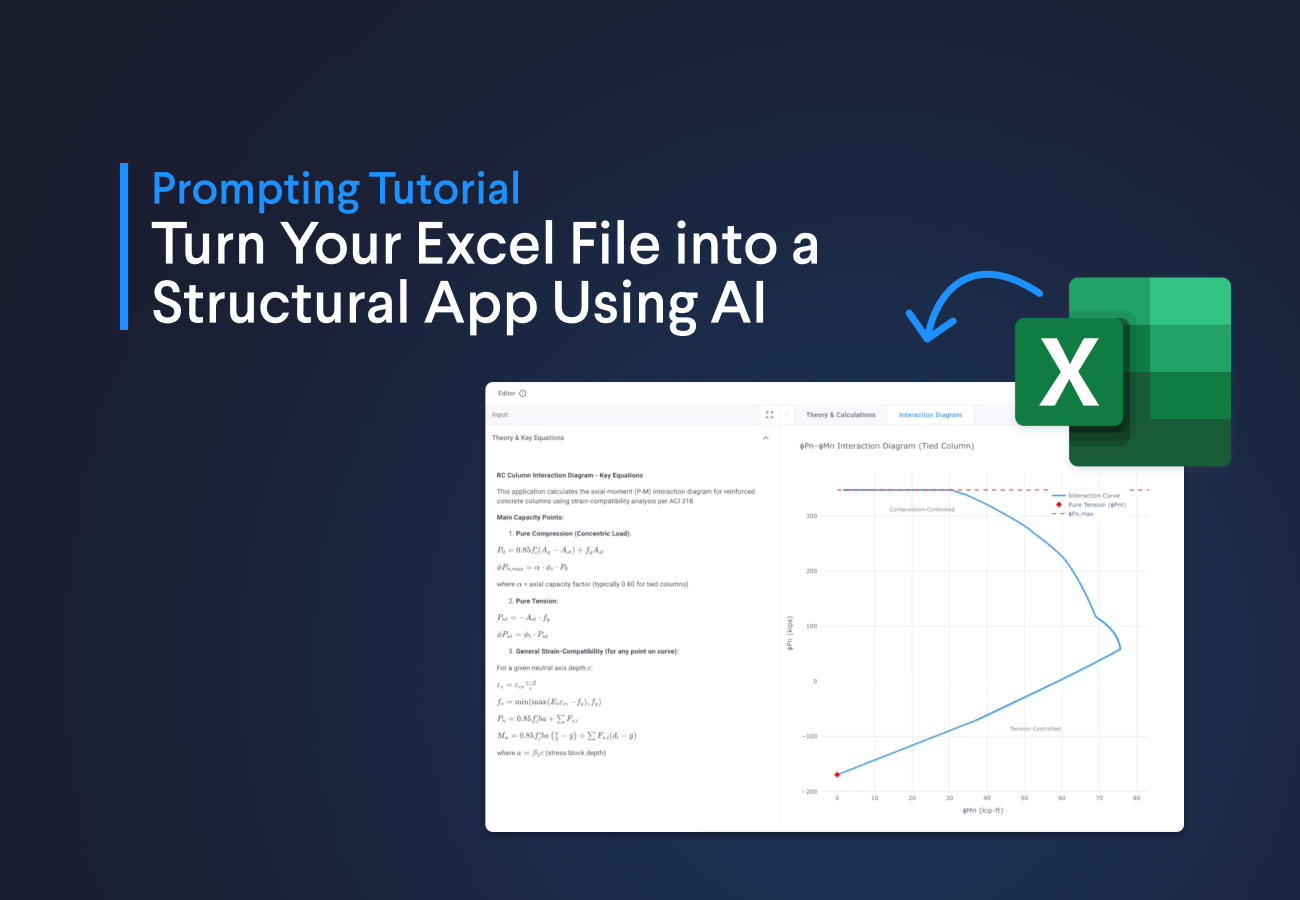
What is a Python Library?

A Python library is a collection of predefined tools that include functions, classes, and modules designed to solve specific tasks without needing to code everything from scratch, saving us time, because in programming, there’s no need to reinvent the wheel.

Moreover, these libraries provide flexibility and customization due to their open source nature, which allows us to explore, modify, and adapt their functionalities according to the specific needs of each project. They also stand out for their ease of use, featuring clear documentation and an active community that makes learning and applying them straightforward, even for those who are not experts in programming.

Some examples of popular Python libraries you may know are NumPy, MatplotLib, Plotly and Pandas. These packages are widely used by engineers but have one common limit. They are not designed for engineering but for data analysis.

However, in this article, I want to share the ones you don't know about yet that are purely for engineers. Let's dive in!

1. Structural modeling and analysis with OpenSeesPy

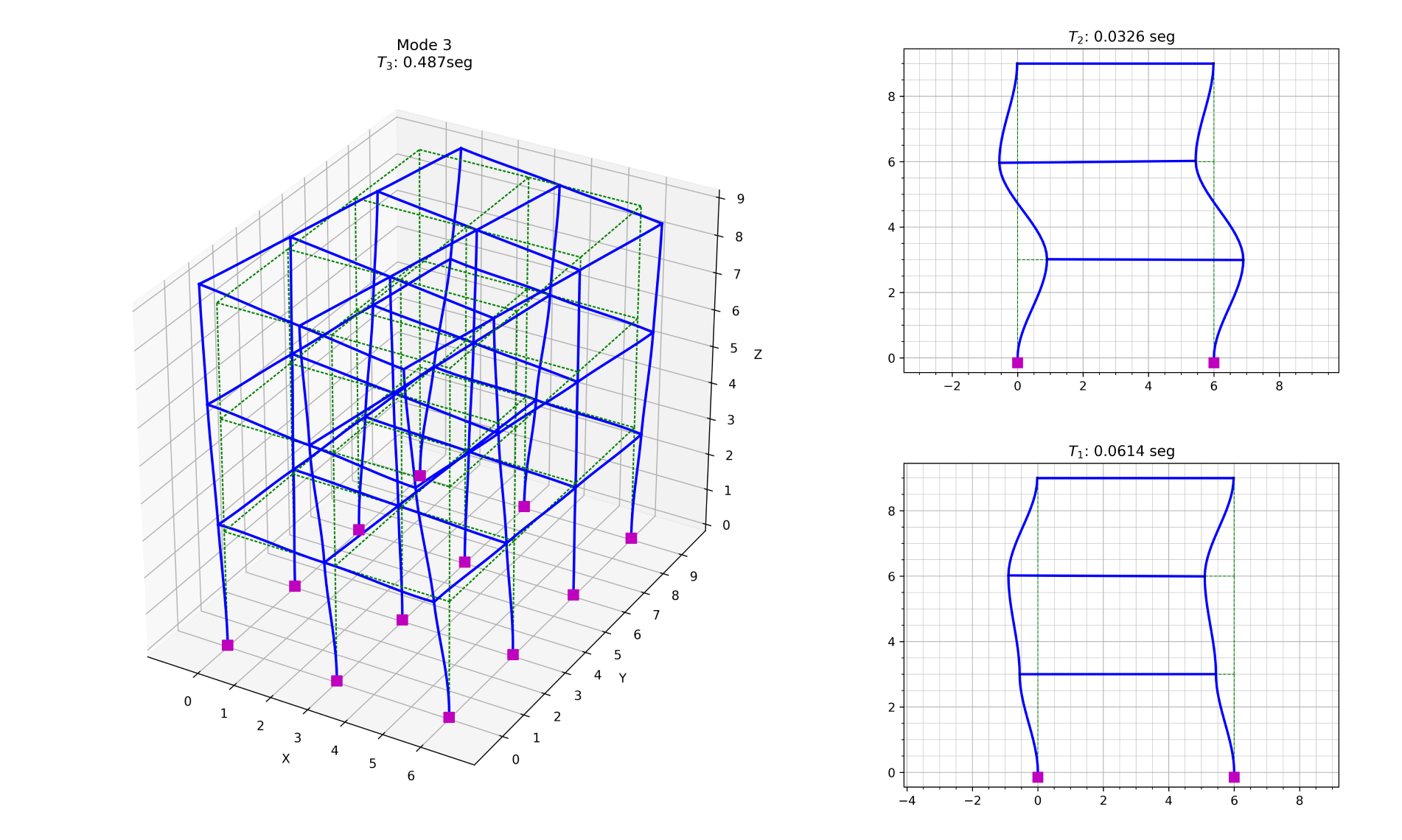
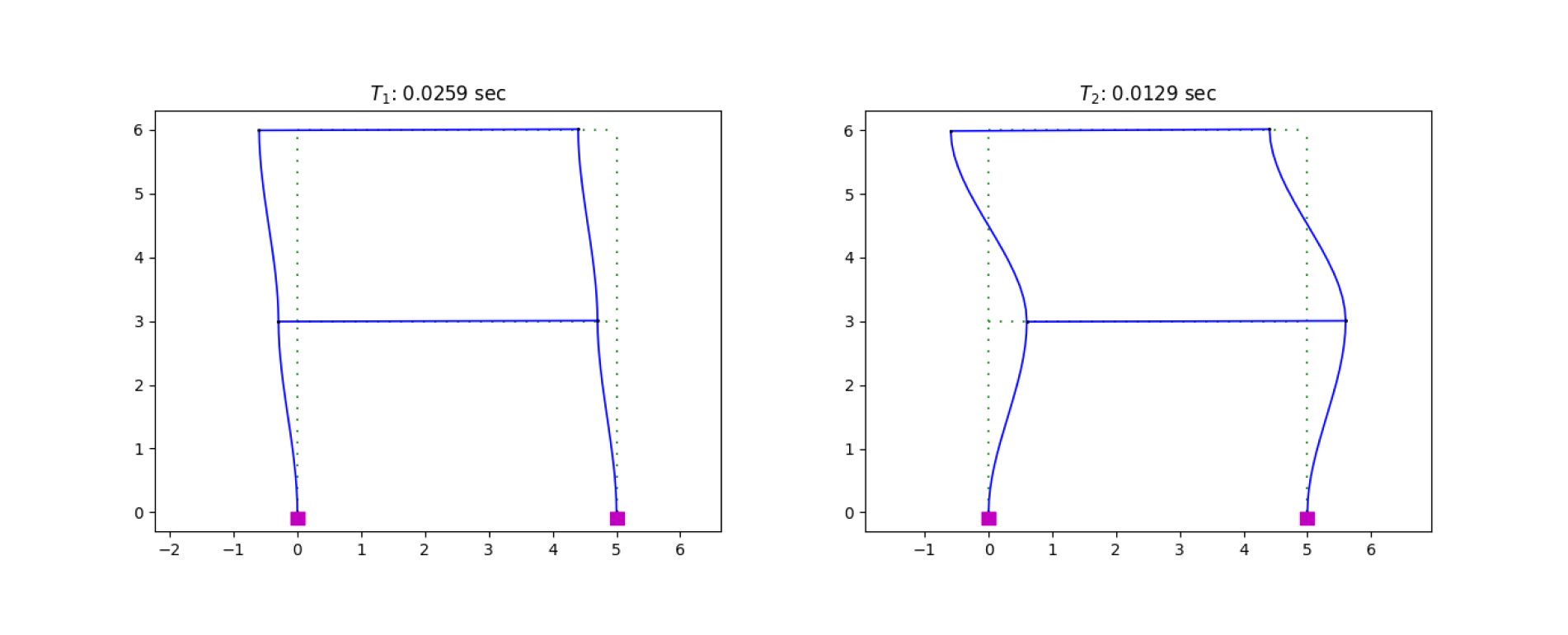
OpenSees is a powerful open-source software. It is ideal for modeling and analyzing structural systems under static and dynamic loads, especially in scenarios involving earthquakes. Its ability to handle nonlinear and advanced analyses makes it particularly useful for seismic engineering projects.

Advantages:

• Advanced modeling: Simulates the plastic behavior of materials and allows for linear analysis, making it a versatile tool for all types of structural projects.
• Dynamic analysis: Supports time-history analysis, spectral modal analysis, and other dynamic analyses with high precision.
• Active community: OpenSees has a large user base that shares examples, models, and solutions to complex problems.

1import openseespy.opensees as ops 
2import opsvis as opsv 
3import matplotlib.pyplot as plt 
4import numpy as np 
5
6ops.wipe() 
7ops.model('basic', '-ndm', 2, '-ndf', 3) 
8
9m = 100             # Mass (kg) 
10h = 3               # Story height (m) 
11L = 5               # Bay width (m) 
12A = 0.09            # Column cross-sectional area (m2) 
13Ic = 0.000675       # Column moment of inertia (m4) 
14Iv = 10e10          # Rigid beam moment of inertia (m4) 
15E = 20e9            # Modulus of elasticity (GPa) 
16
17# Definition of nodes and masses 
18ops.node(1, 0, 0) 
19ops.node(2, L, 0) 
20ops.node(3, 0, 1*h, '-mass', m, 0, 0) 
21ops.node(4, L, 1*h, '-mass', m, 0, 0) 
22ops.node(5, 0, 2*h, '-mass', m/2, 0, 0) 
23ops.node(6, L, 2*h, '-mass', m/2, 0, 0) 
24
25# support 
26ops.fix(1, 1, 1, 1)  # Fixed 
27ops.fix(2, 1, 1, 1)  # Fixed 
28
29ops.geomTransf('Linear', 1) 
30
31# Column 
32ops.element('elasticBeamColumn', 1, 1, 3, A, E, 2*Ic, 1) 
33ops.element('elasticBeamColumn', 2, 2, 4, A, E, 2*Ic, 1) 
34ops.element('elasticBeamColumn', 3, 3, 5, A, E, 1*Ic, 1) 
35ops.element('elasticBeamColumn', 4, 4, 6, A, E, 1*Ic, 1) 
36
37# Beam 
38ops.element('elasticBeamColumn', 5, 3, 4, A, E, Iv, 1) 
39ops.element('elasticBeamColumn', 6, 5, 6, A, E, Iv, 1) 
40
41# Calculation of vibration periods 
42NumModes = 2 
43eigen = np.array(ops.eigen(NumModes)) 
44ω = eigen**0.5 
45T = 2*np.pi/ω 
46
47for i in range(NumModes): 
48    opsv.plot_mode_shape(i+1, endDispFlag=0) 
49    plt.title("$T_{%i}$: %.4f sec" % (i+1, T[i])) 
50plt.show() ```

2. Accessible FEM analysis with PyNite

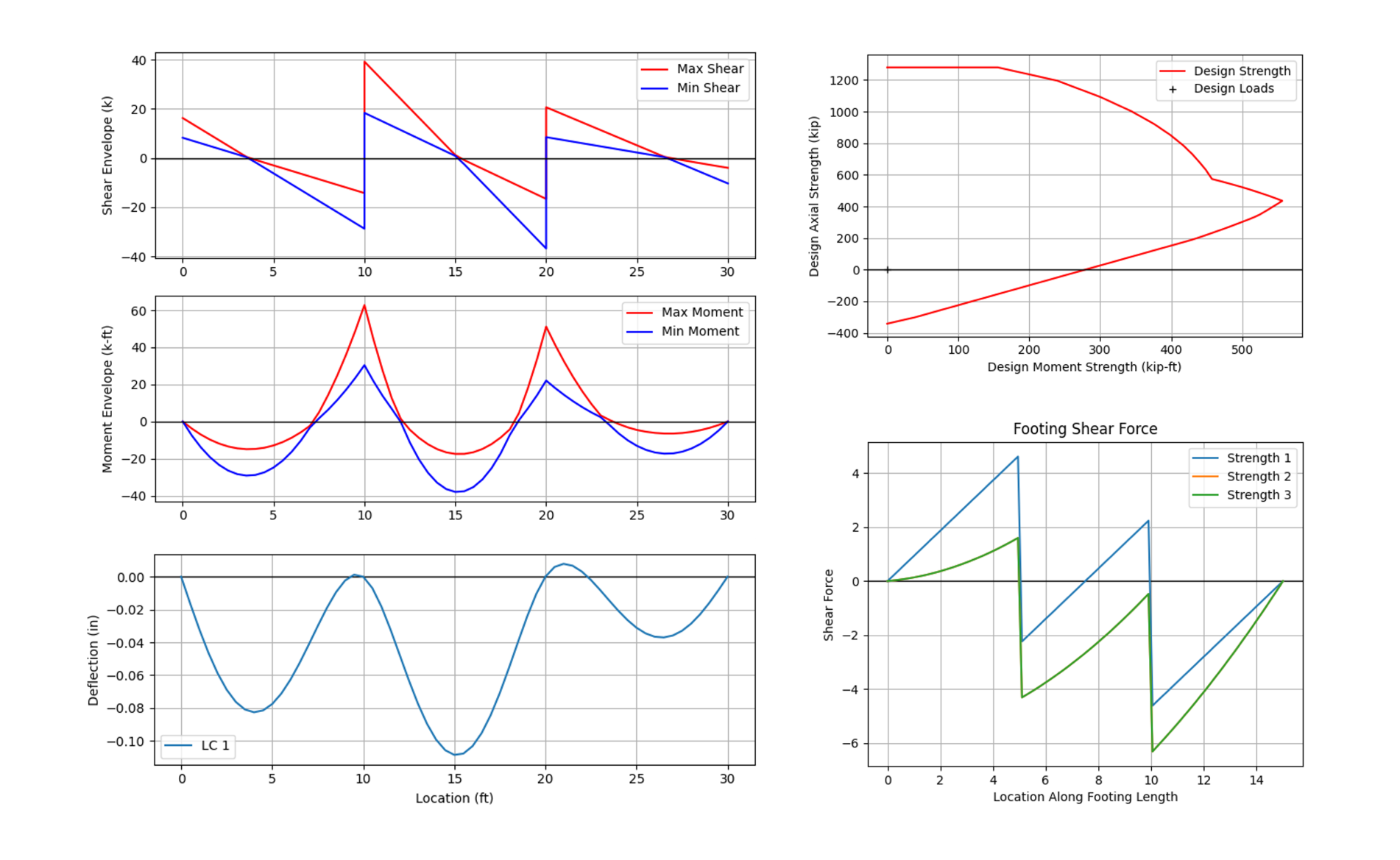
PyNite is a lightweight Python library that allows finite element analysis in a simple and accessible way. Its main goal is to provide a tool that strikes a good balance between simplicity and efficiency for structural engineers who do not need a technically complex solver.

PyNite can perform 3D and 2D static analysis, P-Δ analysis for frame structures, and handle different types of loads: point loads, distributed loads, nodal loads, and load combinations.

Advantages:

• Ease of use: PyNite has a short learning curve, so any engineer with basic programming knowledge can use it.
• Efficient analysis: Perfect for projects where simplicity and speed are required.
• Immediate results: Quickly generates stress and deformation diagrams, allowing you to visualize structural behavior instantly.

1from PyNite import FEModel3D 
2import matplotlib.pyplot as plt 
3mdl = FEModel3D() 
4
5# Add nodes  
6L = 240    # (in) 
7mdl.add_node('N1', 0, 0, 0) 
8mdl.add_node('N2', L, 0, 0) 
9mdl.add_node('N3', 2*L, 0, 0) 
10
11# Material properties 
12E = 29000       # Modulus of elasticity (ksi) 
13G = 11200       # Shear modulus of elasticity (ksi) 
14nu = 0.3        # Poisson's ratio 
15rho = 2.836e-4  # Density (kci) 
16mdl.add_material('Steel', E, G, nu, rho) 
17
18# Add members 
19# Iy = 100 in^4, Iz = 150 in^4 
20# J = 250 in^4 
21# A = 20 in^2 (cross-sectional properties) 
22mdl.add_member('M1', 'N1', 'N2', 'Steel', 100, 150, 250, 20) 
23mdl.add_member('M2', 'N2', 'N3', 'Steel', 100, 150, 250, 20) 
24
25# Supports fixed in x, y, and z translations, free rotation 
26for node in ['N1', 'N2', 'N3']: 
27    mdl.def_support(node, True, True, True, False, False, False) 
28
29# Loads (D: dead load, L: live load) 
30for member in ['M1', 'M2']: 
31    mdl.add_member_dist_load(member, 'Fy', -0.5, -0.5, 0, 240, case='D') 
32    mdl.add_member_dist_load(member, 'Fy', -0.75, -0.75, 0, 240, case='L') 
33
34# Load combinations 
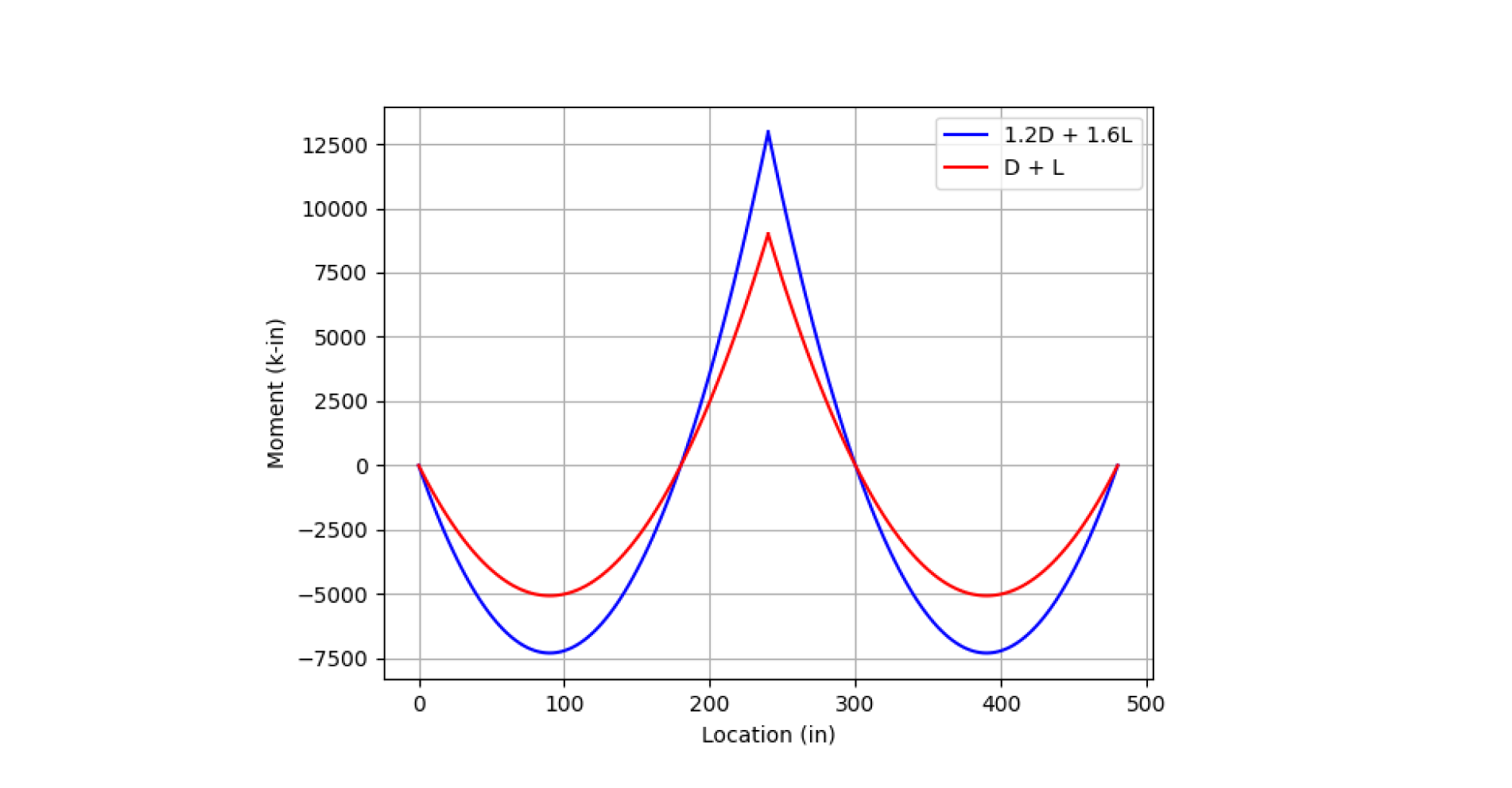
35mdl.add_load_combo('1.2D + 1.6L', {'D': 1.2, 'L': 1.6})  # comb1 = 1.2D + 1.6L 
36mdl.add_load_combo('D + L', {'D': 1.0, 'L': 1.0})        # comb2 = D + L 
37mdl.analyze()  
38
39# Plot the shear diagram with all load combinations 
40x1, M1 = mdl.members['M1'].moment_array("Mz", 100, '1.2D + 1.6L') 
41_, M2 = mdl.members['M1'].moment_array("Mz", 100,'D + L') 
42x2, M3 = mdl.members['M2'].moment_array("Mz", 100, '1.2D + 1.6L') 
43_, M4 = mdl.members['M2'].moment_array("Mz", 100, 'D + L') 
44
45# Plot results 
46# span 1 
47plt.plot(x1, M1, c = 'b', label='1.2D + 1.6L') 
48plt.plot(x1, M2, c = 'r', label='D + L') 
49# span 2
50plt.plot(x2+L, M3, c = 'b') 
51plt.plot(x2+L, M4, c = 'r') 
52plt.xlabel('Location (in)') 
53plt.ylabel('Moment (k-in)') 
54plt.grid(True) 
55plt.legend() 
56plt.show()

3. Calculate cross-sectional properties with SectionProperties

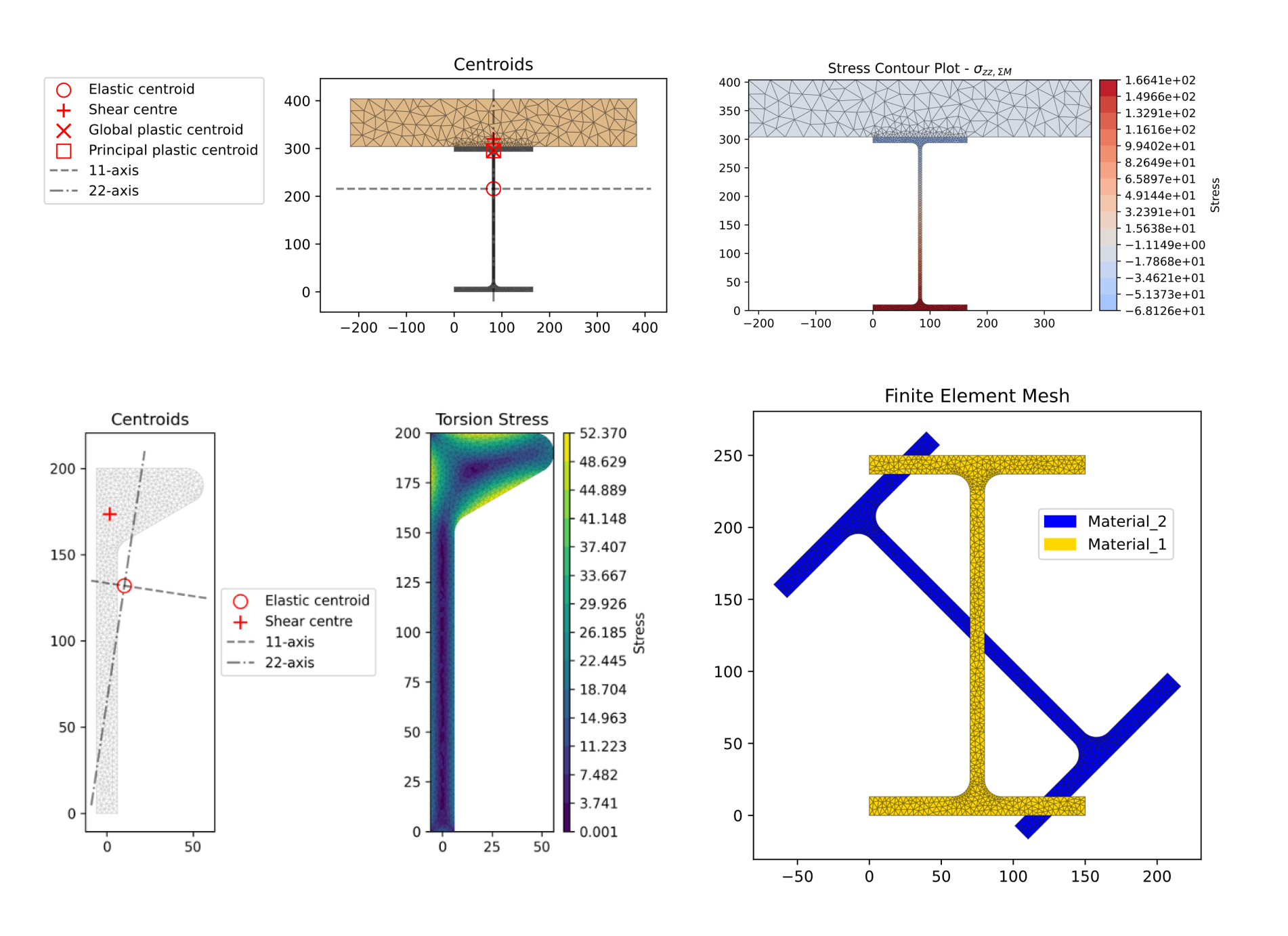
SectionProperties allows the calculation of cross-sectional properties using the finite element method (FEM), such as area, centroid, moments of inertia, bending stresses, and more, making it an essential tool for engineers working with concrete, steel, or timber elements. Additionally, it supports working with .dxf and .3dm (Rhino) files, which is useful for importing geometries from other modeling programs.

One of the impressive features of SectionProperties is its ability to generate precise meshes of cross-sections. Moreover, it provides export options that allow saving calculated geometries and properties in different formats, enabling integration into other workflows.

Advantages:

• Flexibility: Allows the definition of complex sections, including composite and irregular shapes.
• Graphical visualization: Provides a graphical interface to visualize stress and deformation distributions, making it easier to understand the structural behavior of analyzed sections.
• Speed: Performs advanced calculations in seconds, saving time during the preliminary design phase and improving efficiency in project development.
• Accessibility and Open Source: Unlike other commercial tools, SectionProperties is open source and has an available API, making it ideal for researchers as well as engineers needing to customize their workflow.

1import sectionproperties.pre.library.primitive_sections as sections 
2from sectionproperties.analysis.section import Section 
3import matplotlib.pyplot as plt 
4
5# Create outer circular section (diameter = 10) 
6outer_geometry = sections.circular_section(d=10, n=100) 
7
8# Create inner circular section (hole) and shift it (diameter = 4, offset by 2 in x, 1 in y) 
9inner_geometry = sections.circular_section(d=4, n=100) 
10inner_geometry = inner_geometry.shift_section(x_offset=2, y_offset=1) 
11
12# Subtract inner geometry from outer geometry to form a hollow section 
13geometry = outer_geometry - inner_geometry 
14
15# Plot the resulting hollow section 
16geometry.plot_geometry() 
17
18# Generate mesh for the section 
19geometry.create_mesh(mesh_sizes=[1]) 
20
21# Perform section analysis and display results 
22section = Section(geometry, time_info=True) 
23section.display_mesh_info() 
24section.plot_mesh(materials=False) 
25section.calculate_geometric_properties() 
26section.calculate_warping_properties() 
27section.calculate_plastic_properties() 
28section.plot_centroids() 
29section.display_results() 

4. Detailed analysis of reinforced concrete section with ConcreteProperties

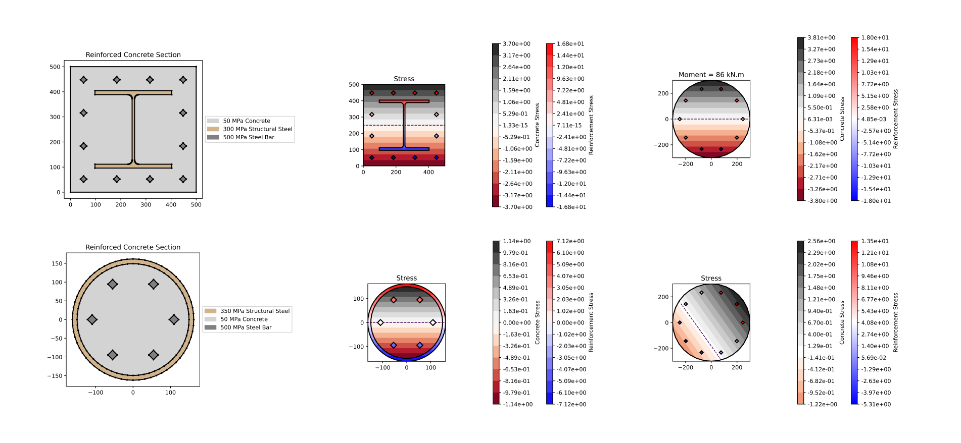
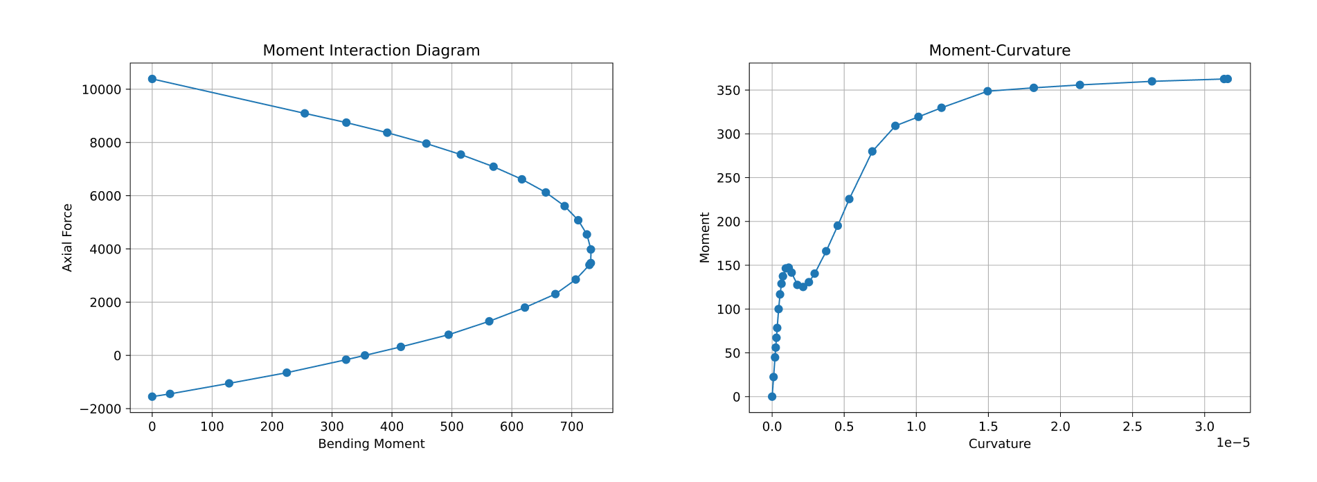
ConcreteProperties facilitates the detailed analysis of reinforced concrete sections, including composite concrete and steel structures as well as prestressed concrete structures.

Unlike SectionProperties, ConcreteProperties specializes in reinforced concrete sections and their detailed analysis. This tool not only allows for the calculation of geometric properties such as cross-sectional area, moments of inertia, centroid, axial stiffness, and more, but it also performs advanced analyses such as moment-curvature and interaction diagrams, which are specifically tailored for the behavior of reinforced concrete under various loading conditions. This makes it the ideal choice when a detailed analysis of the nonlinear behavior of concrete is required, including cracking, ultimate flexural capacity, and effective stiffness under service loads.

Advantages:

• Versatility: ConcreteProperties supports a wide range of materials, from concrete (confined and unconfined) and steel to prestressed material, making it adaptable for different types of projects.
• Specialized analysis: Provides tools for conducting a deep analysis of concrete sections, from initial stiffness to maximum load capacity and service conditions.
• Code compliance: Includes specific modules for validating designs according to standards such as AS3600 and evaluation guidelines like NZS3101, ensuring compliance with recognized standards.
• Clear visualization: Generates detailed graphs that help in understanding structural behavior, including stress distributions and moment-curvature diagrams.

1import matplotlib.pyplot as plt 
2from concreteproperties.design_codes.nzs3101 import NZS3101 
3from concreteproperties.design_codes.as3600 import AS3600 
4from sectionproperties.pre.library.concrete_sections import concrete_rectangular_section 
5from concreteproperties.concrete_section import ConcreteSection 
6from concreteproperties.results import MomentInteractionResults 
7from concreteproperties.results import MomentCurvatureResults 
8
9# Select a design code 
10design_code = NZS3101() 
11# design_code = AS3600() 
12
13# Materials 
14concrete_40 = design_code.create_concrete_material(compressive_strength=40) 
15steel_500 = design_code.create_steel_material(steel_grade="500E")      # steel for design code NZS3101 
16
17# steel_500 = design_code.create_steel_material()                          # steel for design code AS3600 
18geom_col = concrete_rectangular_section( 
19    b=600, d=600, 
20    dia_top=20, area_top=314.16, n_top=4, 
21    dia_bot=20, area_bot=314.16, n_bot=4, 
22    dia_side=20, area_side=314.16, n_side=2, 
23    c_bot=47, c_side=47, c_top=47, 
24    n_circle=8, 
25    conc_mat=concrete_40, steel_mat=steel_500) 
26conc_sec_col = ConcreteSection(geom_col) 
27conc_sec_col.plot_section() 
28design_code.assign_concrete_section(conc_sec_col) 
29f_mi_res, mi_res, phis = design_code.moment_interaction_diagram() 
30ax = MomentInteractionResults.plot_multiple_diagrams( 
31    [f_mi_res, mi_res], ["Factored", "Unfactored"], fmt="-", render=False) 
32
33# design load cases 
34n_stars = [4000e3, 5000e3, -500e3, 1000e3] 
35m_stars = [200e6, 400e6, 100e6, 650e6]
36marker_styles = ["x", "+", "o", "*"] 
37
38# check to see if combination is within diagram and plot result 
39for idx in range(len(n_stars)): 
40    case = f_mi_res.point_in_diagram(n=n_stars[idx], m=m_stars[idx]) 
41    print("Case {num}: {status}".format( 
42        num=idx + 1, status="OK" if case else "FAIL")) 
43    ax.plot(m_stars[idx] / 1e6, n_stars[idx] / 1e3, "k" + marker_styles[idx], 
44            markersize=10, label=f"Case {idx + 1}") 
45ax.legend(loc="lower right") 
46plt.show() 
47
48# Moment-Curvature Analysis 
49moment_curvature_results = conc_sec_col.moment_curvature_analysis() 
50MomentCurvatureResults.plot_results(moment_curvature_results, fmt="-r") 

5. Structural analysis with Anastruct

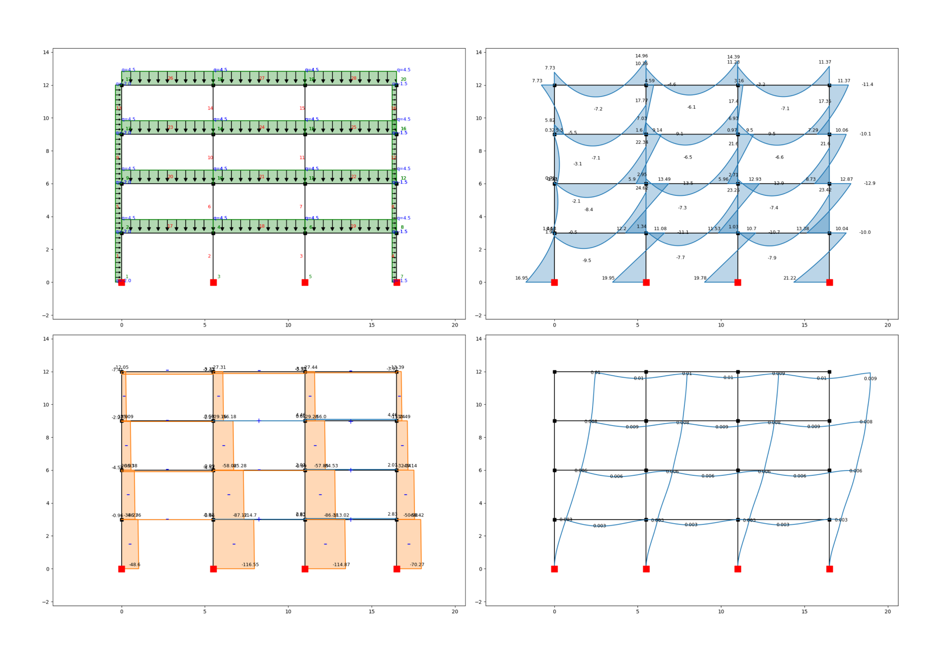
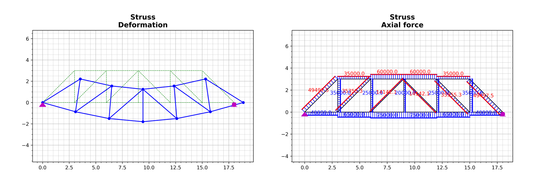
AnaStruct is a lightweight Python library designed to perform linear structural analysis of frames and trusses in 2D, using the finite element method, allowing engineers to quickly obtain clear and precise results without complications.

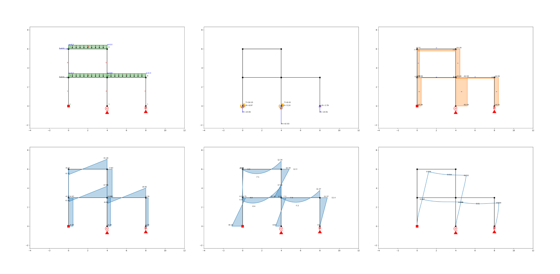
AnaStruct offers a comprehensive set of tools to analyze reactions, bending moments, shear forces, axial forces, and displacements. Additionally, it supports nonlinear nodes and geometric nonlinearity, enhancing its ability to model systems with complex behavior.

Advantages:

• Clear visualization: AnaStruct generates detailed graphs, including bending moment lines, axial forces, shear forces, and displacements, making it easier to interpret and communicate results.
• Ease of use: With straightforward setup, AnaStruct is ideal for engineers looking for a fast and accessible tool for 2D structural calculations.
• Flexibility in section definition: Offers a database of steel profiles such as HEA and IPE, as well as the option to define geometric properties for each element created.

1from anastruct import SystemElements 
2ss = SystemElements(EA=2e4, EI=6e3) 
3
4ss.add_element([[0, 0], [0, 3]]) 
5ss.add_element([[4, 0], [4, 3]]) 
6ss.add_element([[8, 0], [8, 3]]) 
7ss.add_element([[0, 3], [0, 6]]) 
8ss.add_element([[4, 3], [4, 6]]) 
9ss.add_element([[0, 3], [4, 3]]) 
10ss.add_element([[4, 3], [8, 3]]) 
11ss.add_element([[0, 6], [4, 6]]) 
12ss.add_support_fixed(1) 
13
14# Add rotational spring support at node 3 
15ss.add_support_spring(3, translation=3, k=6e3) 
16ss.add_support_spring(5, translation=2, k=3e3) 
17
18# Add loads 
19ss.q_load(q=-6, element_id=[6, 7, 8]) 
20ss.point_load(node_id=[2, 7], Fx=8) 
21ss.solve() 
22ss.show_structure() 
23ss.show_reaction_force() 
24ss.show_axial_force() 
25ss.show_shear_force() 
26ss.show_bending_moment() 
27ss.show_displacement()

Commercial Software APIs

In addition to these open-source libraries, many commercial structural analysis programs offer APIs (Application Programming Interface) that you can use with Python to automate processes. Some of the most well-known are:

• RFEM (Dlubal)
• ETABS (CSI)
• Ansys
• Abaqus
• Tekla

In upcoming blogs, we will explore how to use these APIs to create efficient workflows and automate repetitive tasks in large engineering projects.

What's next?

Using Python is a game changer in structural engineering. If you master the skills to automate your work with Python, you stand out from the crowd. Rather than dealing with repetitive tasks, Python allows you to spend more time creating innovative solutions.

If you want to make your Python automations more accessible, you can use VIKTOR to turn them into intuitive and sharable web apps that further streamline your workflow. With VIKTOR, you can integrate with any third-party software and Python library, boost efficiency and collaboration within engineering teams, and deliver optimal solutions within no time.

Ready to deliver better structural design in less time? Learn more.